Plot Tutorial¶

DegreeDistribution¶

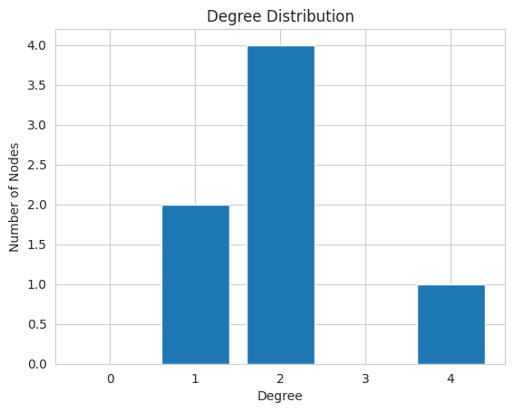
The degreeDistribution of a graph describes the degree (incoming and outgoing edges) that each node has. Networkit.plot.degreeDistribution plots how many nodes of each degree exist within a graph.

We start by creating a graph G.

[2]:

G=nk.Graph(7)
G.addEdge(0,1)
G.addEdge(0,2)
G.addEdge(1,2)
G.addEdge(2,3)
G.addEdge(2,4)
G.addEdge(3,5)
G.addEdge(5,6)

[2]:

True

Plotting the degreeDistribution of a graph G can be done the following way:

[3]:

nk.plot.degreeDistribution(G)

ConnectedComponentsSizes¶

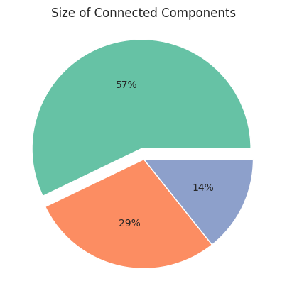
The connectedComponentsSizes describe how many nodes of the graph the individual connected components contain. Networkit.plot.connectedComponentsSizes plots for each indivual component how many nodes of the graph it contains. By default it shows the size relative (as percentages) to the entire population, if relativeSizes is set to False, it shows the absolute number of nodes in each component.

Note: See networkit.components.ConnectedComponents for a description of the algorithm.

For the next example we create a new graph G2 with 3 components: the first component contains the nodes 0-3, the second contains the nodes 4 and 5, and the third contains only node 6 (component of size 1).

[4]:

G2=nk.Graph(7)
G2.addEdge(0,1)
G2.addEdge(1,2)
G2.addEdge(2,3)
G2.addEdge(4,5)

[4]:

True

Plotting the connectedComponentsSizes of a graph G can be done the following way:

[5]:

nk.plot.connectedComponentsSizes(G2, relativeSizes=True)

NodeAttributes¶

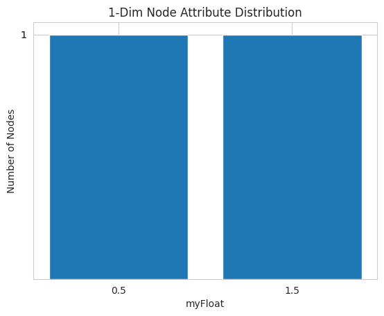
The nodeAttributes are useful in order to efficiently incorporate additional information in the graph data structure.

Note: See networkit.GraphTutorial in section NodeAttributes for a detailed description.

For this example we create a new graph G_attr which contains additional graph attributes.

[6]:

G_attr=nk.Graph(4)
G_attr.addEdge(0,1)
G_attr.addEdge(1,2)
G_attr.addEdge(2,3)
#attaching the attributes to the graph
attrFloat = G_attr.attachNodeAttribute("myFloat", float)
attrStr = G_attr.attachNodeAttribute("myStr", str)
#setting attribute values
attrFloat[0] = 0.5
attrFloat[1] = 1.5
attrStr[1] = "tutorial"
attrStr[2] = "again"

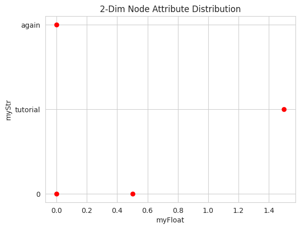
Note: The nk.plot.nodeAttributes can only be called with either one nodeAttribute or a tuple of exactly two nodeAttributes.

• If called with a single nodeAttribute, it plots how frequent each value of the nodeAttribute is present in the graph.

• If called with two nodeAttributes, it plots the 2-Dimensional distribution of the nodes according to the given nodeAttributes

Plotting the nodeAttributes of a graph G can be done the following way:

[7]:

#example with a single attribute
nk.plot.nodeAttributes(G_attr, attrFloat)

#example with two attributes
nk.plot.nodeAttributes(G_attr, (attrFloat, attrStr))

ClusteringPerDegree¶

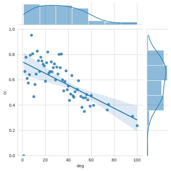
ClusteringPerDegree can be used as centrality measure of the graph. Networkit.plot.ClusteringPerDegree plots for each degree (obtained by DegreeCentrality) the so called Clustering Coefficient (cc) that measures how tight adjacent nodes are clustered together.

For this example we read a medium sized graph given by the networkit.input graphs.

[8]:

# read a graph
G_jazz = nk.readGraph("../input/jazz.graph", nk.Format.METIS)

Note: The pandas library, as well as the seaborn library needs to be installed on your device.

Plotting the ClusteringPerDegree of a graph G can be done the following way:

[9]:

nk.plot.clusteringPerDegree(G_jazz)

CoreDecomposition¶

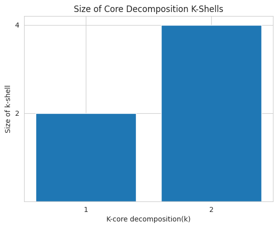
The CoreDecomposition algorithm computes the k-core decomposition of a graph, which is the largest induced subgraph, only consisting of nodes, whose degree is greater than or equal to k. Networkit.plot.coreDecompositionSequence plots the size (number of nodes) of each k-induced subgraph.

See networkit.centrality.coreDecomposition for a description of the algorithm.

For the next example we create a new graph G3, whose k2-shell has size 4 (nodes: 1,3,4,5) and whose k1-shell has size 2 (nodes 0 and 2).

[10]:

G3=nk.Graph(6)
G3.addEdge(0,3) # G3:  0
G3.addEdge(1,3) #      |
G3.addEdge(2,3) #  1 - 3 - 2
G3.addEdge(1,4) #  | X |
G3.addEdge(1,5) #  4 - 5
G3.addEdge(3,4)
G3.addEdge(4,5)
G3.addEdge(3,5)

[10]:

True

Plotting the coreDecompositionSequence of a graph G can be done the following way:

[11]:

nk.plot.coreDecompositionSequence(G3)

HopPlot¶

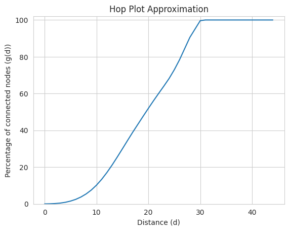
The hopPlot is the set of pairs (d, g(d)) for each natural number d, where g(d) is the fraction of connected node pairs whose shortest connecting path has length at most d. The networkit.plot.hopPlot plots the percentage of connected node pairs, that have a connecting path of length at most d.

Note: The algorithm is approximative. See networkit.distance.hopPlotApproximation for a detailed description of the algorithm.

For this example we read a medium sized graph given by the networkit.input graphs.

[12]:

#larger example
G_big = nk.readGraph("../input/power.graph", nk.Format.METIS)

Plotting the hopPlot of a graph G can be done the following way:

[13]:

nk.plot.hopPlot(G_big)